Exact p-value versus Information Value

As I think I’ve mentioned before, one of the ‘go-to’ stats in my scorecard-building toolkit is the p-value that results from performing Fisher’s Exact Test on contingency tables. It’s straightforward to generate (in most cases), and directly interpretable: it’s just a sum of the probabilities of ‘extreme’ tables. When I started building credit risk scorecards, and using the Information Value (IV) statistic, I had to satisfy myself that there was a sensible relationship between the two values. Now, my combinatoric skills are far too lacking to attempt a rigorous mathematical analysis, so naturally I turn to R and the far easier task of simulating lots of data!

I generated 10,000 2-by-2 tables at random, with cell counts between 5 and 100. Here’s a plot of the (base e) log of the resulting exact p-value, against the log of the IV:

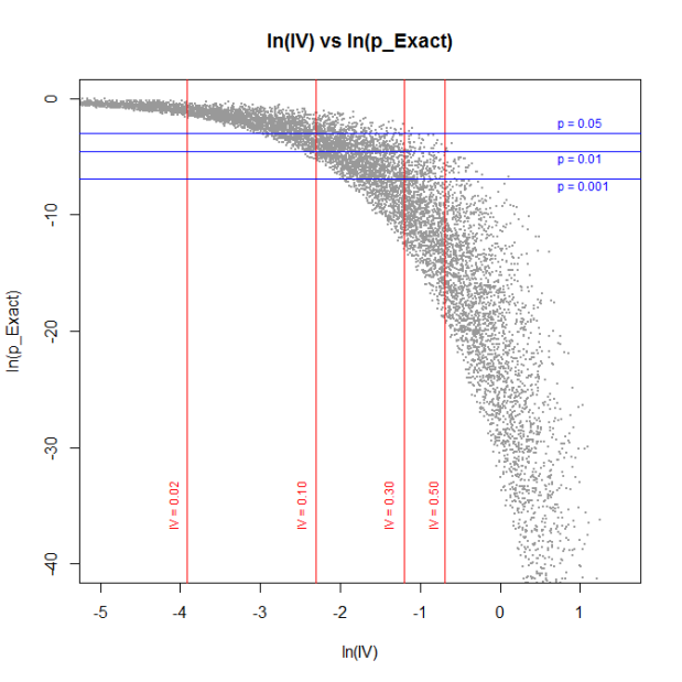
(I’ve taken logs as the relationship is clearer.) As you can see, I’ve drawn in some lines for the typical levels of p-value that people care about (5%, 1% and 0.1%), and the same for the IV (0.02, 0.1, 0.3 and 0.5). In the main, it looks like you’d expect, no glaring outliers.

For fun, I’ll look at those that fall into the area (p_exact > 0.05) and (0.3 < IV < 0.5):

6 29 10 15

p = 0.0751, IV = 0.332

5 84 7 37

p = 0.0613, IV = 0.321

In both cases, the exact p-value says there’s not much evidence that the row/column categories are related to each other — yet the IV tells us there’s “strong evidence”! Of course, the answer is that there’s no one single measure of independence that covers all situations; see, for instance, the famous Anscombe’s Quartet for a visual representation.

Practically, for the situations in which I’m using these measures, it doesn’t matter: if I have at least one indication of significance, I may as well add another candidate variable to the logistic regression that’ll form the basis of my scorecard. If the model selection process doesn’t end up using it, that’s fine.

---

Anyway, I end with a minor mystery. In my previous post, I came up with an upper bound for the IV, which means I can scale my IV to be between zero and one. I presumed that this new scaled version would be more correlated with the exact p-value; after all, how can a relationship with an IV of 0.25, but an upper bound of 5, be less significant than one with an IV of 0.375, but an upper bound of 15 (say)? Proportionally, the former is twice as strong as the latter, no?

What I found was that the scaled version was consistently less correlated! Why would this be? Surely, the scaling is providing more information? I have some suspicions, but nothing concrete at present — hopefully, I can clear this up in a future post.

Upper bound of the Information Value statistic

Information Value

Despite having worked with it for years, it has always irked me that I don’t know the derivation of the Information Value (IV) statistic.

It’s used liberally throughout credit risk work, but the background to its invention seems somewhat hazy. Clearly it’s related to Shannon Entropy, via the construct. In Naeem Siddiqi’s well-known book Credit Risk Scorecards, he writes “Information Value, […] comes from information theory” and references Kulback’s 1959 book Information Theory and Statistics, which I don’t have. Someone else suggested that it stems from the work of I.J. Good, but I can’t find an explicit definition in any of his papers I’ve managed to look at. (I bought his book Good Thinking, about the foundations of probability and statistical interference, but it’s waaaay too complex for me!)

The Information Value (IV) is defined as:

, where is the number of ‘goods’ in category i, and is the number of ‘bads’.

In his book, Siddiqi gives the following rule of thumb regarding the value of IV:

< 0.02	unpredictive
0.02 to 0.1	weak
0.1 to 0.3	medium
0.3 to 0.5	strong
0.5+	“should be checked for over-predicting”

For an independent variable with an IV over 0.5, it might be somehow related to the dependent variable, and you might want to consider leaving it out. (If you build a scorecard that has a bureau score as one of your variables, then you’ll almost certainly see this.)

[See these two links for more about Information Value, and an example or two of its use: All about “Information Value” and Information Value (IV) and Weight of Evidence (WOE).]

Upper Bound

The lower bound of the IV is fairly obviously zero: if for all the categories, then the difference is zero, so their sum is zero times , which is also zero. But what about the upper bound?

I’ve put together this small PDF document: Upper bound of the Information Value (IV), in which (I think!) I show that the upper bound is very close to 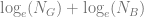, where is the total number of goods, and is the total number of bads.

Of course, it’s wise to at least check the result with some code — so in R, let’s create a million tables at random, and look at the actual figures that are produced:

Z <- 1000000; # number of iterations
IV <- rep(0, Z); # array of IVs
lGB <- rep(0, Z); # array of (log(n_g) + log(n_b))

for (i in 1:Z)
{
	k <- sample(2:20, 1); # number of categories
	g <- sample(1:100, k, replace=T); # good
	b <- sample(1:100, k, replace=T); # bad
	ng <- sum(g);
	nb <- sum(b);
	IV[i] <- sum( ((g/ng)-(b/nb)) * log((g/ng)/(b/nb)) );
	lGB[i] <- log(ng) + log(nb);
}
plot(IV, lGB, xlab="IV", ylab="log(N_G)+log(N_B)",
	main="IV vs log(N_G)+log(N_B)", pch=19,col="blue",cex=0.5);
abline(a=0,b=1,col="red",lwd=2); # draw the line x=y

As you can see, there are no points below the red ‘x=y’ line; in other words, the IV is always less than . There are a few points that are close; the closest is:

min(lGB-IV)
[1] 0.2161227

I know that is not the best possible upper bound — a closer, but more complex answer is reasonably obvious from the document — but “log(number of goods) plus log(number of bads)” is (a) memorable, and (b) close enough for me!