Posts Tagged entropy
Upper bound of the Information Value statistic
Posted by sqlpete in scorecards, stats on February 12, 2017
Information Value
Despite having worked with it for years, it has always irked me that I don’t know the derivation of the Information Value (IV) statistic.
It’s used liberally throughout credit risk work, but the background to its invention seems somewhat hazy. Clearly it’s related to Shannon Entropy, via the 
The Information Value (IV) is defined as:

, where 

In his book, Siddiqi gives the following rule of thumb regarding the value of IV:
| < 0.02 | unpredictive |
| 0.02 to 0.1 | weak |
| 0.1 to 0.3 | medium |
| 0.3 to 0.5 | strong |
| 0.5+ | “should be checked for over-predicting” |
For an independent variable with an IV over 0.5, it might be somehow related to the dependent variable, and you might want to consider leaving it out. (If you build a scorecard that has a bureau score as one of your variables, then you’ll almost certainly see this.)
[See these two links for more about Information Value, and an example or two of its use: All about “Information Value” and Information Value (IV) and Weight of Evidence (WOE).]
Upper Bound
The lower bound of the IV is fairly obviously zero: if 

I’ve put together this small PDF document: Upper bound of the Information Value (IV), in which (I think!) I show that the upper bound is very close to 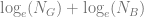


Of course, it’s wise to at least check the result with some code — so in R, let’s create a million tables at random, and look at the actual figures that are produced:
Z <- 1000000; # number of iterations
IV <- rep(0, Z); # array of IVs
lGB <- rep(0, Z); # array of (log(n_g) + log(n_b))

for (i in 1:Z)
{
	k <- sample(2:20, 1); # number of categories
	g <- sample(1:100, k, replace=T); # good
	b <- sample(1:100, k, replace=T); # bad
	ng <- sum(g);
	nb <- sum(b);
	IV[i] <- sum( ((g/ng)-(b/nb)) * log((g/ng)/(b/nb)) );
	lGB[i] <- log(ng) + log(nb);
}
plot(IV, lGB, xlab="IV", ylab="log(N_G)+log(N_B)",
	main="IV vs log(N_G)+log(N_B)", pch=19,col="blue",cex=0.5);
abline(a=0,b=1,col="red",lwd=2); # draw the line x=y
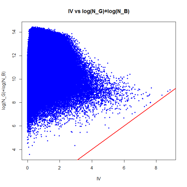
As you can see, there are no points below the red ‘x=y’ line; in other words, the IV is always less than
min(lGB-IV)
[1] 0.2161227
I know that

Recent Comments