Information Value
Despite having worked with it for years, it has always irked me that I don’t know the derivation of the Information Value (IV) statistic.
It’s used liberally throughout credit risk work, but the background to its invention seems somewhat hazy. Clearly it’s related to Shannon Entropy, via the 
The Information Value (IV) is defined as:

, where 

In his book, Siddiqi gives the following rule of thumb regarding the value of IV:
| < 0.02 | unpredictive |
| 0.02 to 0.1 | weak |
| 0.1 to 0.3 | medium |
| 0.3 to 0.5 | strong |
| 0.5+ | “should be checked for over-predicting” |
For an independent variable with an IV over 0.5, it might be somehow related to the dependent variable, and you might want to consider leaving it out. (If you build a scorecard that has a bureau score as one of your variables, then you’ll almost certainly see this.)
[See these two links for more about Information Value, and an example or two of its use: All about “Information Value” and Information Value (IV) and Weight of Evidence (WOE).]
Upper Bound
The lower bound of the IV is fairly obviously zero: if 

I’ve put together this small PDF document: Upper bound of the Information Value (IV), in which (I think!) I show that the upper bound is very close to 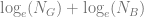


Of course, it’s wise to at least check the result with some code — so in R, let’s create a million tables at random, and look at the actual figures that are produced:
Z <- 1000000; # number of iterations
IV <- rep(0, Z); # array of IVs
lGB <- rep(0, Z); # array of (log(n_g) + log(n_b))

for (i in 1:Z)
{
	k <- sample(2:20, 1); # number of categories
	g <- sample(1:100, k, replace=T); # good
	b <- sample(1:100, k, replace=T); # bad
	ng <- sum(g);
	nb <- sum(b);
	IV[i] <- sum( ((g/ng)-(b/nb)) * log((g/ng)/(b/nb)) );
	lGB[i] <- log(ng) + log(nb);
}
plot(IV, lGB, xlab="IV", ylab="log(N_G)+log(N_B)",
	main="IV vs log(N_G)+log(N_B)", pch=19,col="blue",cex=0.5);
abline(a=0,b=1,col="red",lwd=2); # draw the line x=y
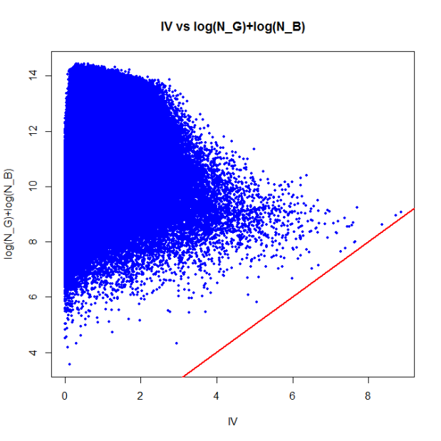
As you can see, there are no points below the red ‘x=y’ line; in other words, the IV is always less than
min(lGB-IV)
[1] 0.2161227
I know that

#1 by Michael Hore on March 25, 2017 - 11:55 am
Interesting topic. I have been tempted to investigate.
I think I found the answer to where this blasted stat was derived! It’s in the first few pages of that information theory book you linked to which is available on Google, in the section on Divergence – this is what would apparently now be called symmetric kullback-leibler divergence according to wikipedia.
Lets say we’re doing WOE/IV on age binning and I will summarize my possibly incorrect understanding. We have our distributions b(age) and g(age) which give the probability that a sample falls in a given age bucket given that they are bad or good respectively.
We start with the Bayes Rule that tells us that LogOdds(Bad:Good given Age) – LogOdds(Bad:Good) = WOE(bad), i.e. your WOE(bad)=log(b(age)/g(age)) gives you a measure of how much you are increasing or decreasing your log odds that the sample is bad when you take into account age vs. when you don’t. WOE(good) is just negative WOE(bad).
The KL(Bad, Good) divergence is the expected WOE(bad), i.e. average change in log-odds by taking into account age, for samples that are actually bad. It’s always positive because on average bad samples are going to be in age buckets where bad is concentrated more than good is concentrated i.e. they end up in buckets with positive WOE, This is intuitively satisfying as well because on average adding data such as age vs. not adding should only ever increase the log-odds in favour of bad for samples that are actually bad, suggesting positive average WOE again. So KL(Bad, Good) is used as a measure of information gained (discriminative power gained) by taking into account age for bad samples.
Symmetric KL is KL(Bad, Good) + KL(Good, Bad), it’s the information gained for samples which are in fact bad plus information gained for samples which are in fact good. It can be written in the form sum((g(age)-b(age))log(g(age)/b(age))) i.e. it is the IV stat.
LikeLike
#2 by sqlpete on March 29, 2017 - 7:55 am
What a great comment – it looks like you’ve nailed it! Thank you very much.
LikeLike
#3 by jayprich on March 4, 2018 - 6:22 pm
The bounded-ness of total information is relevant for “Information Value”, KL grows with sample size whereas WoE is just a log of the ratio.
https://en.wikipedia.org/wiki/Kullback%E2%80%93Leibler_divergence#Discrimination_information
Using the IV criterion will emphasise explaining mid-range probabilities over fitting the tails – for credit worthiness this might not be ideal. This effect is similar to Logistic Regression which also has an underlying robustness and is good at classification, focusing attention on fitting the marginal cases.
If you want to pay more attention to fitting tails to observed data you could stratify the sample or you could use a different link function in your regression – e.g. “probit”.
LikeLike
#4 by sqlpete on April 1, 2018 - 3:44 pm
Very interesting, thank you for your comment!
LikeLike